


Getting agentic AI economics right is less about picking a model and more about picking a pricing plan for the volume you actually expect — proven with numbers, not a vendor’s marketing slide. In this hands-on lab you will build a small, honest cost calculator comparing three ways of processing the same volume of documents: fully-loaded human labor, Bedrock On-Demand pricing, and Bedrock Provisioned Throughput pricing.
You will find the exact breakeven volume where switching from On-Demand to Provisioned Throughput actually saves money. If the economics guide convinced you agentic AI can be cheaper than a human team, this lab is where you calculate whether that is true for your specific volume, not just in general.

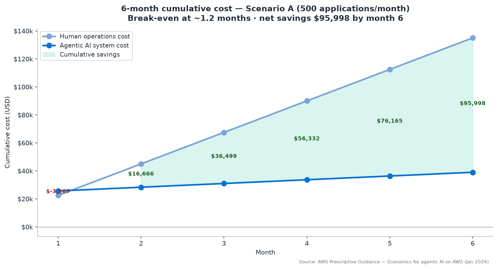
Agentic AI Economics: What You’ll Build
You will build a Python cost-calculator script with three functions — one per cost model — plus a breakeven solver that finds the monthly document volume at which Provisioned Throughput becomes cheaper than On-Demand. Along the way you will walk through the spreadsheet-style logic behind each number by hand first, so the script is a codification of arithmetic you actually understand rather than a black box you copy-pasted.
The worked scenario is a document-processing task: extracting structured fields from inbound vendor invoices, a common enough agentic workload that the same agentic AI economics math generalizes to ticket triage, contract review, or claims processing with different token counts plugged in.
It is worth being explicit about what this calculator deliberately does not model, so you do not mistake its output for a complete financial model: implementation cost (the engineering time to build and validate the extraction pipeline), accuracy-adjusted cost (correcting errors on either side), or the soft costs of a workforce transition.
What it does model precisely is the recurring, steady-state processing cost under each of three pricing structures — which is the number most ROI conversations actually get wrong first, because it is easy to compare a headline On-Demand token price against a wage figure without accounting for either side’s real-world overhead. Get this number right first; the softer costs are real but secondary refinements once the base comparison is trustworthy.
Prerequisites: Python 3.11+, no AWS account strictly required to run the calculator itself (it works from published pricing figures you will look up and hardcode as parameters), though having Bedrock model access helps if you want to measure real token counts on your own documents rather than using the lab’s assumed figures. Budget about 60–75 minutes, most of which is understanding the pricing structure rather than writing code.
Before writing any code, walk the same logic by hand once, spreadsheet-style, so the script that follows codifies numbers you already trust rather than a formula you take on faith. Picture three columns on a whiteboard — Human, On-Demand, Provisioned — each with a monthly total that grows with volume in a different shape.
Human cost grows linearly because every document needs the same four minutes; On-Demand cost also grows linearly, but at a far shallower slope because a token costs a tiny fraction of a cent; Provisioned Throughput cost grows in discrete steps, jumping only when volume crosses a threshold that requires an additional whole Model Unit.
That difference in shape — smooth linear versus stepped — is the entire reason a breakeven volume is worth computing precisely instead of eyeballing a slide.
Agentic AI Economics Walkthrough: Building the ROI Calculator
Step 1 — Define the task and its volume in concrete units
Before any agentic AI economics pricing model means anything, pin down exactly what one unit of work costs in tokens and in human minutes. For this lab, one “document” is an inbound vendor invoice: a human reviewer reads it and keys structured fields (vendor, amount, due date,
line items) into a system in an average of 4 minutes; an LLM-based agent reads the same invoice as roughly 1,800 input tokens (OCR’d text plus a structured-extraction prompt) and produces roughly 350 output tokens (the extracted JSON plus a brief confidence rationale).
TASK = {
    "human_minutes_per_doc": 4,
    "input_tokens_per_doc": 1800,
    "output_tokens_per_doc": 350,
}
Every cost model below is a different way of multiplying this same per-unit cost by volume, so if the per-unit numbers are wrong the comparison is meaningless even when the arithmetic is correct. Get honest numbers here — ideally measured from a real document sample — before trusting anything downstream.
Step 2 — Calculate fully-loaded human labor cost
“Fully-loaded” means wages plus the overhead a business actually pays per employee-hour: payroll taxes, benefits, management overhead, and office/tooling cost — not just the hourly wage. This is the human-side input that agentic AI economics gets wrong most often; a common rule of thumb is a loaded-cost multiplier of roughly 1.3–1.4x base wage for benefits and taxes alone, before adding management overhead.
def human_cost_per_month(volume_docs_per_month, hourly_wage=22.00, loaded_multiplier=1.35):
    """
    hourly_wage: base wage for a document-processing reviewer role.
    loaded_multiplier: accounts for payroll tax, benefits, and overhead.
    """
    loaded_hourly_rate = hourly_wage * loaded_multiplier
    hours_needed = (volume_docs_per_month * TASK["human_minutes_per_doc"]) / 60
    return hours_needed * loaded_hourly_rate


for volume in [1_000, 10_000, 100_000, 1_000_000]:
    cost = human_cost_per_month(volume)
    print(f"{volume:>9,} docs/mo -> human labor: ${cost:,.2f}")
Skipping the loaded multiplier is a common way vendors quietly stack the deck: a bare hourly wage understates true labor cost by a third or more once payroll taxes and benefits are included. A realistic loaded rate is what makes the comparison defensible to a finance stakeholder.
Step 3 — Look up and hardcode Bedrock On-Demand pricing structure
Amazon Bedrock’s On-Demand pricing model charges per token processed, with separate rates for input tokens and output tokens, varying by model and AWS Region — you pay only for what you use, with no capacity commitment and no minimum. For this lab,
use representative per-million-token rates for a mid-tier Claude model on Bedrock (check the live Bedrock pricing page for your target model and region before using these numbers for a real business decision — token pricing changes over time and by model).
ON_DEMAND_PRICING = {
    "input_per_million_tokens": 3.00,   # USD per 1M input tokens, representative mid-tier model rate
    "output_per_million_tokens": 15.00, # USD per 1M output tokens
}

def on_demand_cost_per_month(volume_docs_per_month):
    input_tokens = volume_docs_per_month * TASK["input_tokens_per_doc"]
    output_tokens = volume_docs_per_month * TASK["output_tokens_per_doc"]

    input_cost = (input_tokens / 1_000_000) * ON_DEMAND_PRICING["input_per_million_tokens"]
    output_cost = (output_tokens / 1_000_000) * ON_DEMAND_PRICING["output_per_million_tokens"]

    return input_cost + output_cost


for volume in [1_000, 10_000, 100_000, 1_000_000]:
    cost = on_demand_cost_per_month(volume)
    print(f"{volume:>9,} docs/mo -> On-Demand: ${cost:,.2f}")
Output tokens are consistently priced higher than input tokens on Bedrock, since generating a token costs more than reading one. An input-heavy, output-light task like this one looks meaningfully cheaper under On-Demand than a task with the reverse ratio — modeling the two token types separately keeps the calculator accurate for your specific task shape.
Step 4 — Look up and model Bedrock Provisioned Throughput pricing structure
Provisioned Throughput works differently, and getting this pricing structure right matters for agentic AI economics at scale: instead of paying per token, you purchase a number of Model Units (MUs) for a committed duration — no commitment, one month, or six months, with longer commitments priced at a discount — and each MU gives you a fixed maximum input and output token-per-minute throughput capacity,
billed hourly whether or not you actually use that capacity. This is the critical economic difference from On-Demand: Provisioned Throughput cost is a function of committed capacity, not consumed volume.
PROVISIONED_PRICING = {
    "hourly_rate_per_mu_no_commitment": 21.50,   # representative rate, no-commitment tier
    "hourly_rate_per_mu_1_month": 17.00,          # representative rate, 1-month commitment
    "hourly_rate_per_mu_6_month": 13.50,          # representative rate, 6-month commitment
    "tokens_per_minute_per_mu": 200_000,           # representative combined input+output throughput per MU
}

def provisioned_cost_per_month(volume_docs_per_month, commitment="1_month"):
    rate_key = f"hourly_rate_per_mu_{commitment}"
    hourly_rate = PROVISIONED_PRICING[rate_key]

    total_tokens_per_month = volume_docs_per_month * (
        TASK["input_tokens_per_doc"] + TASK["output_tokens_per_doc"]
    )
    # Assume traffic is spread across a 22-business-day, 10-hour operating window,
    # which determines the peak tokens-per-minute the provisioned capacity must sustain.
    operating_minutes_per_month = 22 * 10 * 60
    required_tokens_per_minute = total_tokens_per_month / operating_minutes_per_month

    mus_needed = max(1, -(-required_tokens_per_minute // PROVISIONED_PRICING["tokens_per_minute_per_mu"]))  # ceiling division

    hours_per_month = 22 * 10  # billed hourly for the whole commitment window, not just active hours
    return mus_needed * hourly_rate * hours_per_month, mus_needed


for volume in [1_000, 10_000, 100_000, 1_000_000]:
    cost, mus = provisioned_cost_per_month(volume)
    print(f"{volume:>9,} docs/mo -> Provisioned (1-mo): ${cost:,.2f} ({mus:.0f} MUs)")
Provisioned Throughput is sold in whole Model Units, not fractional capacity — a workload needing 1.2 MUs is billed for 2. That lumpiness is exactly what makes Provisioned Throughput uneconomical at low volume, and it is why the breakeven in Step 5 needs an actual calculation rather than a rule of thumb.
Step 5 — Find the breakeven volume with a solver, not a guess
Rather than eyeballing a chart, sweep a range of volumes and find the crossover point where the Provisioned Throughput cost curve drops below the On-Demand cost curve — remembering that because of the MU ceiling from Step 4, the “breakeven” is a step function, not a smooth line, so report a range rather than a single number.
def find_breakeven(commitment="1_month", max_volume=2_000_000, step=1_000):
    crossover_volume = None
    for volume in range(step, max_volume + step, step):
        od_cost = on_demand_cost_per_month(volume)
        pt_cost, _ = provisioned_cost_per_month(volume, commitment=commitment)
        if pt_cost < od_cost and crossover_volume is None:
            crossover_volume = volume
            break
    return crossover_volume


for commitment in ["no_commitment", "1_month", "6_month"]:
    breakeven = find_breakeven(commitment=commitment)
    print(f"Breakeven volume ({commitment}): {breakeven:,} docs/month")
The MU ceiling from Step 4 is a discontinuous step function, so a closed-form algebraic solution either handles that explicitly or is slightly wrong near the boundary. A brute-force sweep across realistic volumes sidesteps that entirely and is easy for a reviewer to audit line by line.
Step 6 — Compare all three models side by side across a volume range
Assemble a single table that a non-technical stakeholder can read in one glance: for each volume tier, the agentic AI economics of the workload — cost of each model and which one wins.
def build_comparison_table(volumes):
    rows = []
    for volume in volumes:
        human = human_cost_per_month(volume)
        on_demand = on_demand_cost_per_month(volume)
        provisioned, mus = provisioned_cost_per_month(volume, commitment="1_month")

        cheapest = min(
            [("Human labor", human), ("On-Demand", on_demand), ("Provisioned (1-mo)", provisioned)],
            key=lambda pair: pair[1],
        )

        rows.append({
            "volume": volume,
            "human": human,
            "on_demand": on_demand,
            "provisioned": provisioned,
            "provisioned_mus": mus,
            "cheapest": cheapest[0],
        })
    return rows


table = build_comparison_table([1_000, 5_000, 10_000, 25_000, 50_000, 100_000, 250_000, 500_000, 1_000_000])
for row in table:
    print(
        f"{row['volume']:>9,} | human ${row['human']:>10,.0f} | "
        f"on-demand ${row['on_demand']:>10,.0f} | "
        f"provisioned ${row['provisioned']:>10,.0f} ({row['provisioned_mus']:.0f} MU) | "
        f"cheapest: {row['cheapest']}"
    )
The human-labor column is the number that actually justifies building an agentic system in the first place. If both Bedrock options cost more than the human baseline at your volume, the honest conclusion is that automation is not yet an economic win — leaving that baseline out of the table is how ROI calculations become marketing instead of analysis.
Step 7 — Model batch inference as a fourth option where applicable
If your document-processing workload does not need real-time responses — invoices can reasonably be processed in a nightly or hourly batch rather than the instant an email arrives — Amazon Bedrock's batch inference mode is worth modeling too as a fourth lever in the agentic AI economics comparison, since it is priced at a meaningful discount versus On-Demand for select models.
BATCH_DISCOUNT = 0.50  # batch mode costs roughly 50% less than On-Demand for eligible models

def batch_cost_per_month(volume_docs_per_month):
    return on_demand_cost_per_month(volume_docs_per_month) * (1 - BATCH_DISCOUNT)


for volume in [10_000, 100_000, 1_000_000]:
    print(f"{volume:>9,} docs/mo -> Batch: ${batch_cost_per_month(volume):,.2f}")
Batch and Provisioned Throughput solve distinct problems: Provisioned Throughput buys guaranteed low-latency capacity, while batch trades away latency guarantees for a straight discount. For overnight invoice processing where nobody is waiting on the response, batch mode can beat both other options on pure cost — skipping it would understate how cheap the agentic option can get.
Step 8 — Sanity-check the calculator against a real invoice sample
Before presenting any agentic AI economics numbers to a stakeholder, validate the assumed token counts from Step 1 against a small real sample rather than trusting an estimate. Run ten to twenty representative invoices through your actual extraction prompt and record real token usage from the Bedrock response metadata.
import boto3
import json

bedrock_runtime = boto3.client("bedrock-runtime", region_name="us-east-1")

def measure_real_token_usage(invoice_text, extraction_prompt_template):
    prompt = extraction_prompt_template.format(invoice_text=invoice_text)
    body = json.dumps({
        "anthropic_version": "bedrock-2023-05-31",
        "max_tokens": 500,
        "messages": [{"role": "user", "content": prompt}],
    })
    response = bedrock_runtime.invoke_model(
        modelId="anthropic.claude-3-5-sonnet-20241022-v2:0",
        body=body,
    )
    result = json.loads(response["body"].read())
    usage = result.get("usage", {})
    return usage.get("input_tokens"), usage.get("output_tokens")
The entire calculator rests on the token estimates from Step 1, which are easy to get wrong by 2x or more if real invoices are longer or more variable than assumed — enough to point the breakeven conclusion at the wrong pricing model entirely. Measuring real usage on even a small sample is the single highest-leverage validation step in this lab.
Step 9 — Export results to CSV and chart the crossover visually
A table of numbers convinces an engineer; a chart with a visible crossing line convinces a room full of stakeholders in the first ten seconds of a meeting. Export the comparison table from Step 6 to CSV, then render a simple line chart with the three cost curves and a vertical marker at the breakeven volume from Step 5.
import csv

def export_comparison_csv(rows, filename="agentic_ai_economics_comparison.csv"):
    with open(filename, "w", newline="") as f:
        writer = csv.DictWriter(f, fieldnames=["volume", "human", "on_demand", "provisioned", "provisioned_mus", "cheapest"])
        writer.writeheader()
        for row in rows:
            writer.writerow(row)
    print(f"Wrote {filename}")


export_comparison_csv(table)
import matplotlib.pyplot as plt

def plot_cost_curves(volumes, breakeven_volume):
    human = [human_cost_per_month(v) for v in volumes]
    on_demand = [on_demand_cost_per_month(v) for v in volumes]
    provisioned = [provisioned_cost_per_month(v, commitment="1_month")[0] for v in volumes]

    plt.figure(figsize=(9, 5))
    plt.plot(volumes, human, label="Human labor (fully loaded)")
    plt.plot(volumes, on_demand, label="Bedrock On-Demand")
    plt.plot(volumes, provisioned, label="Bedrock Provisioned Throughput (1-mo)")
    plt.axvline(x=breakeven_volume, color="gray", linestyle="--", label=f"Breakeven ~{breakeven_volume:,}")
    plt.xlabel("Documents per month")
    plt.ylabel("Monthly cost (USD)")
    plt.title("Agentic AI Economics: Cost Comparison by Volume")
    plt.legend()
    plt.tight_layout()
    plt.savefig("agentic_ai_economics_chart.png", dpi=150)
    print("Saved chart: agentic_ai_economics_chart.png")


volumes_to_plot = list(range(1_000, 1_000_001, 5_000))
breakeven = find_breakeven(commitment="1_month")
plot_cost_curves(volumes_to_plot, breakeven)
The point of a breakeven volume is to communicate it to whoever approves the Provisioned Throughput purchase, and most of those people will not read a script or CSV line by line. A chart showing the human-labor line well above both Bedrock options, with a clearly marked crossing point, makes the lab's conclusion legible in the time it takes to glance at a slide.
Agentic AI Economics: Common Mistakes to Avoid
Every one of these mistakes distorts the agentic AI economics calculation enough to flip a go/no-go decision — each has the same shape: a number that looks reasonable in isolation quietly biases the comparison toward whichever conclusion the model's builder already expected. Watch for these specifically when doing agentic AI economics for your own workload, especially before presenting the result to a stakeholder who will make a real budget decision on it.
- Comparing bare hourly wage to token cost instead of fully-loaded labor cost. Skipping the loaded multiplier from Step 2 is the single most common way agentic AI economics gets overstated; it inflates the apparent savings by a third or more, which does not survive contact with a finance team's actual cost model.
- Treating Provisioned Throughput MUs as fractional capacity. Model Units are whole units — a workload needing 1.3 MUs worth of throughput is billed for 2, not 1.3. Forgetting the ceiling function from Step 4 systematically underestimates Provisioned Throughput cost.
- Assuming Provisioned Throughput is always cheaper at "high" volume without computing the actual breakeven. The crossover point in Step 5 depends heavily on your specific token counts, commitment term, and operating-hours assumption — no universal volume threshold applies to every agentic AI economics workload.
- Ignoring commitment-term risk. A 6-month Provisioned Throughput commitment is billed hourly for the full term whether or not volume holds steady — a seasonal or declining workload can turn a sound agentic AI economics breakeven calculation into a bad financial commitment if volume drops after you commit.
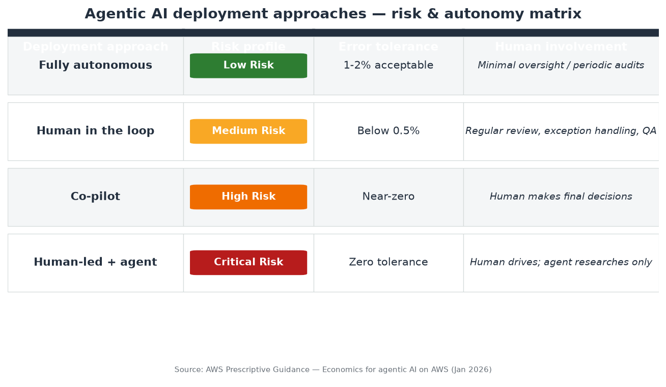
Agentic AI Economics: Going Further — Modeling Risk and Hybrid Strategies
For the authoritative reference on this topic, see the official Amazon Bedrock pricing page.
The calculator above answers "what does this cost at a given volume," which is necessary but not sufficient for a real agentic AI economics purchasing decision — real workloads do not sit at a single steady volume all year.
The most valuable extension is modeling volume variance: run the calculator across a distribution of plausible volumes (a low month, a typical month, a fiscal-quarter-end peak) and compute the blended annual cost under each pricing model instead of one month's snapshot.
A Provisioned Throughput commitment that looks like a clear win at your "typical" volume can look considerably worse once you weight in the low months where you still pay for committed capacity you are not using — the single biggest risk a single-point breakeven calculation hides.
A second extension is a hybrid strategy instead of an all-or-nothing choice. Many production deployments run a baseline Provisioned Throughput commitment sized to the low-to-typical end of their volume distribution, capturing the discount on steady-state load, and burst to On-Demand for peak-volume days that would otherwise require idle over-provisioned capacity.
Extend the calculator with a "baseline MU count" parameter: route volume up to that baseline through the Provisioned Throughput function and everything above it through On-Demand, then compare the hybrid total against each pure strategy across your volume distribution — this hybrid is very often the actual economic optimum, and it is invisible if you only ever compare the two pricing models as mutually exclusive.
The third extension is a sensitivity table on the token-count assumption from Step 1. Since Step 8 established that real invoices vary in length, rerun the Step 6 comparison table at 1,400, 1,800, and 2,400 input tokens per document to see how much your breakeven conclusion depends on that single input.
If the breakeven volume moves dramatically, the conclusion is fragile and worth validating with a larger sample before committing budget; if it barely moves, present the conclusion with much higher confidence.
A worked example makes the volume-variance extension concrete. Suppose a typical month processes 60,000 invoices, fiscal-quarter-end months spike to 140,000, and the slowest month drops to 35,000. A single-point calculation run only against the 60,000-invoice figure might show Provisioned Throughput winning comfortably.
But a 6-month commitment sized for that volume still bills the full committed Model Units in the 35,000-invoice slow month, while the 140,000-invoice peak may exceed committed capacity and spill onto On-Demand pricing anyway.
Multiply the Provisioned Throughput monthly cost by 12, sum the On-Demand cost across each month at its own realistic volume, and compare the two annual totals — it is common to find the annualized comparison favors a lower commitment tier or a hybrid approach even when a single month's snapshot favored a larger commitment.
Finally, this lab's cost model counts inference only. A production agentic pipeline also carries the AgentOps instrumentation costs covered in the companion lab — CloudWatch Logs ingestion, custom metrics, and alarms — plus whatever orchestration compute ties the pieces together.
None of that is large enough to change which pricing model wins at a given volume, but it is large enough that a finance stakeholder will ask about it, so build a small fixed monthly overhead line into the final comparison table rather than presenting pure inference cost as the whole story.
Agentic AI Economics: Frequently Asked Questions
These are the questions finance and engineering teams raise together once they take this lab's calculator into a real budget conversation about agentic AI economics.
Is Provisioned Throughput ever worth it below the calculated breakeven volume?
Rarely on cost alone within an agentic AI economics model, but sometimes on latency or capacity guarantees — Provisioned Throughput exists partly to guarantee a fixed throughput ceiling that On-Demand's shared capacity cannot promise during traffic spikes. If your workload has hard latency SLAs independent of cost, that is a separate justification from the pure ROI calculation in this lab.
Why does the breakeven volume change if I change the commitment term from 1 month to 6 months?
Longer commitments carry a lower hourly rate per Model Unit in exchange for the reduced flexibility of a longer lock-in, so the same throughput capacity costs less per hour under a 6-month term than a 1-month term — which pulls the agentic AI economics breakeven volume lower (Provisioned Throughput wins at a smaller volume) but increases the financial risk described in the Going Further section if volume drops during the commitment.
What is the biggest single risk in committing to Provisioned Throughput based on this calculator?
Volume assumptions that do not hold. Every agentic AI economics breakeven calculation assumes a steady monthly volume; the risk-modeling extension in Going Further exists specifically because real workloads fluctuate, and a 6-month commitment sized for a typical month becomes expensive idle capacity during a slow month.
How does batch inference change the breakeven calculation from Step 5?
It adds a fourth option that frequently beats both On-Demand and Provisioned Throughput on pure cost for latency-tolerant workloads, as modeled in Step 7 of the agentic AI economics calculator. It does not change the On-Demand vs. Provisioned Throughput breakeven itself, but it often makes that specific comparison moot for workloads where a batch window is acceptable.
Does the human labor comparison assume 100% accuracy from the reviewer, and 100% accuracy from the agent?
No, and this is an intentional simplification worth flagging rather than hiding: this lab's calculator compares raw processing cost,
not error-adjusted cost. A complete economic model would also weight in the cost of correcting errors on each side — human transcription mistakes versus model extraction mistakes — which typically requires its own measurement exercise (a sampled accuracy audit against ground truth) rather than an assumption, and is a natural next extension once the base cost comparison in this lab is validated.
This lab turned agentic AI economics from a slide-deck argument into a script you can run against your own numbers: three cost functions — human labor, Bedrock On-Demand,
and Bedrock Provisioned Throughput — swept across a volume range to find the exact breakeven point where committed capacity starts paying for itself. The honest version of this exercise always includes the human-labor baseline, always validates token assumptions against real samples, and always models volume risk before committing to a multi-month Provisioned Throughput term.