


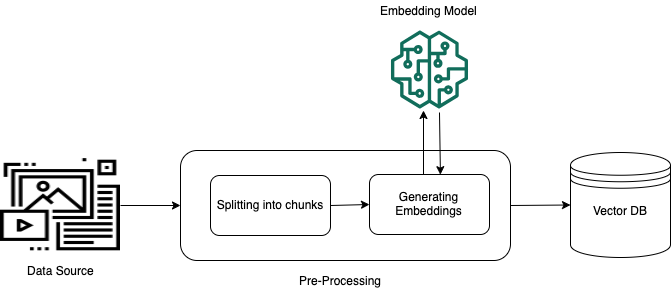
In this hands-on lab you will build a working vector database two different ways for the same product-search scenario: Amazon OpenSearch Service with a k-NN vector index, and Amazon RDS for PostgreSQL with the pgvector extension. You will load identical sample product embeddings into both vector database engines, run a similarity search against each, and compare setup effort and query latency side by side.

What You’ll Build: A Vector Database Comparison Lab
By the end of this lab you will have a small, runnable product-search proof of concept backed by two separate vector database engines. You’ll stand up an OpenSearch domain with a k-NN-enabled index, and separately an RDS for PostgreSQL instance with pgvector installed.
Then you’ll insert the same eight sample product embeddings into each vector database and run an identical “find similar products” query against both, recording wall-clock latency and the number of manual steps each path required.
This lab assumes you already understand the concepts from the parent tutorial, AWS Vector Database & RAG — what embeddings are and why similarity search matters for retrieval-augmented generation. Here we go hands-on with two real vector database options.
Prerequisites: an AWS account with permissions to create OpenSearch domains and RDS instances, the AWS CLI configured with credentials, Python 3.9+ with boto3 and psycopg2-binary installed, and roughly 45-60 minutes (OpenSearch domain creation alone takes 10-15 minutes). Everything here uses small, low-cost instance sizes — destroy both resources when you’re done to avoid ongoing charges.
You’ll also want the requests and requests_aws4auth packages for signing requests to OpenSearch’s HTTPS endpoint, since it authenticates with AWS Signature Version 4 rather than a username and password. The official opensearch-py client wraps this signing step for you, but we use raw requests calls here so every request stays visible while you learn how this particular vector database handles authentication.
Step 1: Create an OpenSearch Domain (or Serverless Collection)
OpenSearch Service is the managed search-engine option for a vector database. For a lab, a provisioned domain with a single small data node is the fastest way to get a stable endpoint; OpenSearch Serverless is the better choice for spiky production traffic, but it adds its own network-policy and collection concepts.
We’ll use a provisioned domain here for clarity, and note the Serverless path where it differs.
aws opensearch create-domain \
  --domain-name product-vectors-lab \
  --engine-version "OpenSearch_2.13" \
  --cluster-config InstanceType=t3.small.search,InstanceCount=1 \
  --ebs-options EBSEnabled=true,VolumeType=gp3,VolumeSize=10 \
  --node-to-node-encryption-options Enabled=true \
  --encryption-at-rest-options Enabled=true \
  --domain-endpoint-options EnforceHTTPS=true \
  --access-policies '{
    "Version": "2012-10-17",
    "Statement": [{
      "Effect": "Allow",
      "Principal": {"AWS": "*"},
      "Action": "es:*",
      "Resource": "arn:aws:es:us-east-1:ACCOUNT_ID:domain/product-vectors-lab/*"
    }]
  }'
The open access policy above is only acceptable because this is a throwaway lab domain behind your own AWS credentials; in production you would scope the resource policy to an IAM role or front the domain with fine-grained access control and a VPC endpoint. Domain creation takes 10-15 minutes — poll status before moving on.
We also left the domain publicly reachable rather than placing it inside a VPC: a VPC-attached domain needs a subnet, security group, and a bastion host or Session Manager tunnel just to reach it from your laptop, tripling setup time without changing the k-NN mechanics this lab teaches.
If you later adapt this lab into a real project, moving the domain into a private subnet is one of the first hardening steps to take — we revisit this in the Going Further section.
If you’d rather try OpenSearch Serverless, the equivalent setup is an aws opensearchserverless create-collection call with type=VECTORSEARCH, plus a network policy and encryption policy created beforehand. Serverless collections scale compute automatically and bill by OpenSearch Compute Units, which suits bursty traffic well, but the extra policy objects mean more setup steps than the provisioned domain used here. Both paths converge again at index creation in Step 2.
aws opensearch describe-domain \
  --domain-name product-vectors-lab \
  --query 'DomainStatus.{Processing:Processing,Endpoint:Endpoints}'
Once Processing reports false and an endpoint is populated, capture it — you’ll use it for every request in this lab.
Step 2: Create the k-NN Vector Database Index
Unlike a relational table, an OpenSearch index needs the index.knn setting turned on at creation time, plus a field mapped as type knn_vector with a fixed dimension. This tells the vector database to build an approximate nearest-neighbor graph (HNSW) for that field instead of treating it as an ordinary array.
Our sample product embeddings are 8-dimensional toy vectors — real embedding models like Amazon Titan Text Embeddings produce 1024 or 1536 dimensions, but a small dimension keeps this lab fast and easy to eyeball.
import boto3
import requests
from requests_aws4auth import AWS4Auth

region = "us-east-1"
service = "es"
credentials = boto3.Session().get_credentials()
awsauth = AWS4Auth(
    credentials.access_key, credentials.secret_key, region, service,
    session_token=credentials.token,
)

host = "https://search-product-vectors-lab-XXXXXXXX.us-east-1.es.amazonaws.com"

index_body = {
    "settings": {"index.knn": True},
    "mappings": {
        "properties": {
            "product_id": {"type": "keyword"},
            "name": {"type": "text"},
            "embedding": {
                "type": "knn_vector",
                "dimension": 8,
                "method": {
                    "name": "hnsw",
                    "engine": "faiss",
                    "space_type": "cosinesimil",
                    "parameters": {"ef_construction": 128, "m": 24},
                },
            },
        }
    },
}

resp = requests.put(f"{host}/products-knn", auth=awsauth, json=index_body)
print(resp.status_code, resp.text)
We chose the faiss engine with HNSW because it’s the current recommended default for most workloads — it balances recall and speed well. Cosine similarity (cosinesimil) is the standard space type for text/product embeddings since magnitude usually doesn’t carry meaning.
The two HNSW parameters, ef_construction and m, control the shape of the nearest-neighbor graph built at index time: m is how many bidirectional links each node keeps, and ef_construction is how wide a candidate list the algorithm explores while building those links. Higher values improve recall at the cost of slower indexing and more memory — 128/24 is a reasonable middle ground for a lab.
There is a matching query-time parameter, ef_search, which trades query latency for recall without rebuilding the index.
Run a quick sanity check that the index accepted the mapping before moving on — a typo in the method block fails silently in some client libraries and only surfaces once you try to query.
curl -s -X GET "$host/products-knn/_mapping" --aws-sigv4 "aws:amz:us-east-1:es" | python3 -m json.toolStep 3: Create the RDS for PostgreSQL Instance
Now the relational path. RDS for PostgreSQL ships pgvector as a pre-installed, trusted extension on supported engine versions (PostgreSQL 13 through 17), so there’s no custom parameter group or shared_preload_libraries change required in the common case — a non-superuser database user can simply run CREATE EXTENSION. If your account uses rds.allowed_extensions to lock down which extensions can be installed, add vector to that allowlist first via a parameter group.
aws rds create-db-instance \
  --db-instance-identifier product-vectors-lab \
  --db-instance-class db.t4g.micro \
  --engine postgres \
  --engine-version 16.4 \
  --master-username labadmin \
  --master-user-password 'ChangeMe-Lab-Password1' \
  --allocated-storage 20 \
  --storage-type gp3 \
  --publicly-accessible \
  --backup-retention-period 0
We disabled backups (--backup-retention-period 0) purely because this is a disposable lab instance; never do that for anything you intend to keep. Wait for the instance to become available before connecting.
aws rds wait db-instance-available --db-instance-identifier product-vectors-lab
aws rds describe-db-instances \
  --db-instance-identifier product-vectors-lab \
  --query 'DBInstances[0].Endpoint.Address' --output text
RDS instance provisioning typically takes 5-10 minutes for a single-AZ micro instance — noticeably faster than the OpenSearch domain in Step 1, your first data point for the complexity comparison later in this lab. We picked db.t4g.micro and single-AZ deployment purely for lab cost.
A production deployment supporting real product-search traffic would typically use a larger, non-burstable instance class (db.r6g or db.r7g memory-optimized families are common for a vector database workload, since HNSW indexes are held in memory) and Multi-AZ for automatic failover. We also left --publicly-accessible on so this lab works from a laptop — treat that exactly like the OpenSearch access policy in Step 1: acceptable for a disposable lab, not for anything holding real data.
Step 4: Enable pgvector and Create the Vector Database Table
Connect with psql or psycopg2, enable the extension, then create a table with a vector column sized to match your embedding dimension.
import psycopg2

conn = psycopg2.connect(
    host="product-vectors-lab.XXXXXXXX.us-east-1.rds.amazonaws.com",
    port=5432,
    dbname="postgres",
    user="labadmin",
    password="ChangeMe-Lab-Password1",
)
conn.autocommit = True
cur = conn.cursor()

cur.execute("CREATE EXTENSION IF NOT EXISTS vector;")

cur.execute("""
    CREATE TABLE IF NOT EXISTS products (
        product_id  TEXT PRIMARY KEY,
        name        TEXT NOT NULL,
        embedding   vector(8)
    );
""")
print("pgvector enabled and products table ready")
Notice how much shorter this vector database setup is than the OpenSearch index setup — that’s the core tradeoff you’re evaluating in this lab. pgvector gives you a familiar SQL table with one extra column type, while OpenSearch requires learning its own settings and mapping DSL.
One connection detail worth calling out: we authenticated with a plain master-user password for lab simplicity, but RDS for PostgreSQL also supports IAM database authentication, which lets your application connect using short-lived tokens generated from an IAM role instead of a stored password — swapping it in only changes how the connection is authenticated, not the SQL that follows.
Confirm the extension actually loaded before moving on, since a typo in the extension name (pgvector instead of vector) fails with a clear but easy-to-miss error.
cur.execute("SELECT extname, extversion FROM pg_extension WHERE extname = 'vector';")
print(cur.fetchone())
Step 5: Load Identical Sample Product Embeddings Into Both Stores
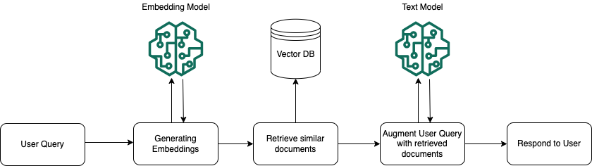
To keep this lab fast and reproducible without calling a real embedding model, we’ll use eight small fixed 8-dimensional vectors standing in for product embeddings. In a real pipeline you would generate these with Amazon Bedrock’s Titan Text Embeddings model (amazon.titan-embed-text-v2:0) via bedrock-runtime.invoke_model, which returns a 1024-dimension float array per product description — the loading code below would be identical, just with longer vectors.
products = [
    {"product_id": "p1", "name": "Wireless noise-cancelling headphones",
     "embedding": [0.12, 0.98, 0.44, 0.31, 0.07, 0.65, 0.22, 0.53]},
    {"product_id": "p2", "name": "Over-ear studio headphones",
     "embedding": [0.14, 0.95, 0.41, 0.29, 0.09, 0.61, 0.25, 0.50]},
    {"product_id": "p3", "name": "Bluetooth in-ear earbuds",
     "embedding": [0.20, 0.90, 0.38, 0.35, 0.11, 0.58, 0.30, 0.47]},
    {"product_id": "p4", "name": "Stainless steel coffee grinder",
     "embedding": [0.88, 0.10, 0.05, 0.92, 0.77, 0.15, 0.60, 0.09]},
    {"product_id": "p5", "name": "Drip coffee maker with timer",
     "embedding": [0.85, 0.14, 0.08, 0.89, 0.74, 0.18, 0.57, 0.12]},
    {"product_id": "p6", "name": "Espresso machine, dual boiler",
     "embedding": [0.90, 0.08, 0.03, 0.95, 0.80, 0.11, 0.63, 0.06]},
    {"product_id": "p7", "name": "Running shoes, lightweight mesh",
     "embedding": [0.40, 0.45, 0.85, 0.20, 0.33, 0.90, 0.15, 0.70]},
    {"product_id": "p8", "name": "Trail running shoes, waterproof",
     "embedding": [0.38, 0.48, 0.82, 0.23, 0.36, 0.87, 0.18, 0.68]},
]
The vectors are grouped so that similar products (headphones, coffee machines, running shoes) sit close together in the fake vector space — this makes it easy to verify the similarity queries in Step 6 return sensible results. Load them into OpenSearch first, using the bulk API for efficiency even at this tiny scale.
bulk_lines = []
for p in products:
    bulk_lines.append(f'{{"index":{{"_index":"products-knn","_id":"{p["product_id"]}"}}}}')
    bulk_lines.append(str(p).replace("'", '"'))
bulk_body = "\n".join(bulk_lines) + "\n"

resp = requests.post(
    f"{host}/_bulk",
    auth=awsauth,
    data=bulk_body,
    headers={"Content-Type": "application/x-ndjson"},
)
print(resp.status_code, resp.json().get("errors"))
Now load the same eight records into PostgreSQL. The pgvector Python integration accepts a plain Python list cast to vector — no bulk API concept needed, just a standard executemany.
insert_sql = "INSERT INTO products (product_id, name, embedding) VALUES (%s, %s, %s) ON CONFLICT (product_id) DO NOTHING;"
rows = [(p["product_id"], p["name"], p["embedding"]) for p in products]
cur.executemany(insert_sql, rows)
print(f"Inserted {len(rows)} rows into pgvector table")
Both inserts above are idempotent by design — OpenSearch uses each product’s product_id as the document _id, and the pgvector insert uses ON CONFLICT ... DO NOTHING against the primary key. That matters in a real ingestion pipeline, where a network blip mid-batch is common and you don’t want a retry to silently double-count products.
Step 6: Run a Similarity Query Against Both Stores
With data loaded, query both stores for products similar to a new “wireless earbuds” query embedding. In OpenSearch, k-NN queries use the knn query clause with a k parameter for how many nearest neighbors to return.
import time

query_vector = [0.16, 0.93, 0.40, 0.33, 0.08, 0.60, 0.26, 0.51]

knn_query = {
    "size": 3,
    "query": {"knn": {"embedding": {"vector": query_vector, "k": 3}}},
}

start = time.perf_counter()
resp = requests.post(f"{host}/products-knn/_search", auth=awsauth, json=knn_query)
opensearch_latency_ms = (time.perf_counter() - start) * 1000
results = resp.json()["hits"]["hits"]
for hit in results:
    print(hit["_source"]["name"], hit["_score"])
print(f"OpenSearch query latency: {opensearch_latency_ms:.1f} ms")
In pgvector, similarity search is plain SQL using a distance operator — <-> for Euclidean distance, <=> for cosine distance, or <#> for negative inner product. We used cosine similarity on the OpenSearch side, so we match it here with <=>, ordering ascending because it returns cosine *distance* (lower is more similar).
start = time.perf_counter()
cur.execute(
    "SELECT product_id, name, embedding <=> %s::vector AS distance "
    "FROM products ORDER BY distance ASC LIMIT 3;",
    (query_vector,),
)
pg_results = cur.fetchall()
pg_latency_ms = (time.perf_counter() - start) * 1000
for row in pg_results:
    print(row)
print(f"pgvector query latency: {pg_latency_ms:.1f} ms")
At this toy scale (8 rows, no HNSW index on the pgvector column) both queries should return the same three headphone products in the same order, and both should complete in well under 50ms — the comparison becomes interesting only at production scale, which is why the “Going Further” section below focuses on indexing and cost at scale rather than these micro-benchmarks.
Real product search almost always needs to combine similarity with a metadata filter — “find similar headphones under $50,” for example. Both approaches below assume you’ve added a numeric price field alongside the embedding.
# OpenSearch: combine k-NN with a filter clause
filtered_knn_query = {
    "size": 3,
    "query": {
        "knn": {
            "embedding": {
                "vector": query_vector,
                "k": 3,
                "filter": {"range": {"price": {"lte": 50}}},
            }
        }
    },
}
resp = requests.post(f"{host}/products-knn/_search", auth=awsauth, json=filtered_knn_query)
# pgvector: an ordinary WHERE clause alongside the distance ORDER BY
cur.execute(
"SELECT product_id, name, embedding <=> %s::vector AS distance "
"FROM products WHERE price <= 50 ORDER BY distance ASC LIMIT 3;",
(query_vector,),
)This is where the two engines diverge in developer ergonomics: the pgvector version is a filter clause any SQL developer already knows, while the OpenSearch version requires learning that filter nests inside the knn clause specifically so the engine can apply it efficiently during the graph search rather than as a slow post-filter over the full result set.
Step 7: Compare Vector Database Setup Complexity and Query Ergonomics
With both pipelines running, step back and compare what each path actually required. OpenSearch needed a domain (10-15 min provisioning), an access-policy decision, a custom index mapping with engine/method/space-type choices, request signing, and NDJSON bulk formatting — five distinct new concepts. RDS for PostgreSQL needed an instance (5-10 min provisioning), one CREATE EXTENSION statement, an ordinary CREATE TABLE, and standard SQL — effectively zero new concepts if you already know PostgreSQL.
The gap narrows once you add filters and joins, which is where pgvector's "it's just SQL" advantage compounds: you can join the products table against orders, inventory, or pricing tables in the same query as the similarity search. OpenSearch can filter too, but joining across indexes the way a relational database joins tables is not something it's built for.
That gap is exactly why pgvector is often the first choice for teams already running a relational database, while an OpenSearch vector database earns its extra setup cost once you need hybrid search, very high query throughput, or centralized search infrastructure across multiple data types.
It's worth being honest about where this comparison cuts the other way: OpenSearch's mapping and method configuration is more upfront work, but it buys you built-in support for combining vector similarity with full-text relevance scoring, aggregations, and horizontal scale-out — capabilities that would require substantially more custom engineering to replicate in PostgreSQL alone.
If your product-search use case is likely to grow into "search bar with typo tolerance, filters, facets, and semantic re-ranking all in one query," that future is much closer to OpenSearch's native feature set than pgvector's.
Step 8: Clean Up Both Resources
Both resources in this lab bill continuously while they exist, so tear them down as soon as you've finished comparing results. Deleting the OpenSearch domain and the RDS instance are both single CLI calls.
aws opensearch delete-domain --domain-name product-vectors-lab

aws rds delete-db-instance \
  --db-instance-identifier product-vectors-lab \
  --skip-final-snapshot \
  --delete-automated-backups
We passed --skip-final-snapshot because this is disposable lab data; omit that flag for any instance holding real data so RDS takes a final snapshot before deletion. Both delete operations run asynchronously — poll describe-domain or describe-db-instances if you want to confirm they've fully terminated.
Common Mistakes
These are the pitfalls most learners hit the first time they wire up either vector database, based on the exact steps in this lab.
- Forgetting
index.knn: trueat index creation. If you create the OpenSearch index without this setting and only add the field mapping, k-NN queries will fail or silently fall back to a brute-force scan — the setting cannot be added to an existing index without reindexing. - Dimension mismatch between the index/table and the embedding model. A
knn_vectorfield or a pgvector column locks in a fixed dimension at creation time. Switching from an 8-dimension toy vector to a real 1024-dimension Titan embedding later means recreating the vector database index or table, not just re-inserting data. - Skipping an HNSW index on the pgvector column at scale. A bare
vectorcolumn with no index works fine for 8 rows but forces a full sequential scan at 100,000+ rows; forgetting to add anivfflatorhnswindex on the column is the single most common pgvector performance mistake. - Not tearing down both resources after the lab. An OpenSearch t3.small domain and an RDS db.t4g.micro instance are both billed continuously once created — delete the domain and instance when you're finished, not just when you stop querying them.
Going Further: Indexing at Scale and Cost Hardening
The eight-row lab above intentionally hides the real differences between these two vector database engines, which only appear at scale. On the pgvector side, add an approximate-nearest-neighbor index once your table grows past a few thousand rows — an hnsw index trades a small amount of recall for dramatically faster queries, the same tradeoff OpenSearch's HNSW graph makes internally.
cur.execute(
    "CREATE INDEX ON products USING hnsw (embedding vector_cosine_ops) "
    "WITH (m = 16, ef_construction = 64);"
)
print("HNSW index created on pgvector column")
On the OpenSearch side, production hardening means moving off a single data node, enabling fine-grained access control instead of an open resource policy, and — if traffic is spiky — considering OpenSearch Serverless so you stop paying for idle capacity between bursts.
An idle RDS db.t4g.micro instance is typically cheaper per month than an idle OpenSearch t3.small domain with equivalent storage, but OpenSearch's advantage grows once you need hybrid keyword+vector search, since it can combine BM25 text relevance with k-NN in a single query — something pgvector cannot do natively without pairing it with PostgreSQL full-text search and manually blending scores.
Add basic error handling around both clients before calling this production-ready: retry transient 5xx responses from the OpenSearch _bulk endpoint with backoff, and wrap the psycopg2 connection in a context manager or connection pool (e.g. psycopg2.pool.SimpleConnectionPool) so a dropped connection doesn't take down the whole ingestion job.
import time

def bulk_with_retry(host, awsauth, bulk_body, max_attempts=4):
    for attempt in range(1, max_attempts + 1):
        resp = requests.post(
            f"{host}/_bulk",
            auth=awsauth,
            data=bulk_body,
            headers={"Content-Type": "application/x-ndjson"},
        )
        if resp.status_code < 500 and resp.status_code != 429:
            return resp
        wait_seconds = 2 ** attempt
        print(f"Bulk attempt {attempt} got {resp.status_code}, retrying in {wait_seconds}s")
        time.sleep(wait_seconds)
    raise RuntimeError("Bulk indexing failed after retries")
On monitoring, both engines expose the metrics you'd want before trusting either vector database in production. OpenSearch domains publish CloudWatch metrics like ClusterStatus.red, SearchLatency, and KNNGraphMemoryUsage — the last one matters because HNSW graphs live in JVM off-heap memory, and running out of it degrades k-NN recall before it causes outright failures.
RDS for PostgreSQL publishes CPUUtilization, FreeableMemory, and ReadLatency/WriteLatency through CloudWatch as well, plus Performance Insights if you enable it, which is the more useful tool for spotting a pgvector query that's fallen back to a sequential scan.
On cost: for this lab's tiny instance sizes, expect the OpenSearch t3.small.search domain and the RDS db.t4g.micro instance to cost roughly the same low single-digit dollars per day if left running, with OpenSearch typically a bit higher once you add the EBS-backed storage overhead most k-NN indexes need.
At production scale the two diverge more — one more reason teams default to a pgvector-based vector database when their workload doesn't specifically need OpenSearch's hybrid search or multi-index scale-out.
Frequently Asked Questions
Which is faster, OpenSearch k-NN or pgvector?
At the tiny scale in this lab, neither — both return in single-digit to low double-digit milliseconds because there's no meaningful data volume to stress either vector database index. At real scale (hundreds of thousands to millions of vectors) both can be fast if properly indexed with HNSW; the practical difference shows up more in operational concerns like hybrid search, sharding strategy, and behavior under concurrent write load than in raw single-query latency.
Do I need to change a parameter group to enable pgvector on RDS?
Not in the default case. pgvector ships as a pre-installed, trusted PostgreSQL extension on current RDS PostgreSQL versions, so a non-superuser database user can run CREATE EXTENSION vector; directly. You only need a parameter group change if your account restricts installable extensions via rds.allowed_extensions, in which case you'd add vector to that allowlist first.
What happens if the dimension of my query vector doesn't match the index or table?
Both engines reject the request. OpenSearch returns a mapping/dimension error on the knn query, and pgvector raises a PostgreSQL error such as "different vector dimensions" when you try to compare or insert a vector of the wrong length against a fixed-dimension vector(n) column. Always confirm your embedding model's output dimension matches what you declared when you created the vector database index or table.
Should I run both stores in production, or pick one?
Most teams pick one vector database per use case rather than running both permanently. This lab runs both side by side purely so you can compare them directly; in production, choose pgvector when your data and queries are already relational and you want ordinary SQL joins/filters alongside similarity search, and choose OpenSearch when you need hybrid keyword+vector search, very high query throughput, or you're already standardized on OpenSearch elsewhere in your stack.
Why did my OpenSearch k-NN query return fewer than k results?
This usually happens when a filter is applied after the nearest-neighbor search rather than inside the knn clause's filter parameter, as covered in the mistakes section above. It can also happen with very small datasets like this lab's eight rows combined with an aggressive filter — if fewer than three products satisfy the filter, you simply won't get three results back, which is expected behavior rather than a bug.
You've now built the same product-search scenario on two different vector database engines: an OpenSearch k-NN index and an RDS pgvector table, loaded with identical sample embeddings and queried for nearest neighbors.
The provisioning time, query syntax, and operational tradeoffs you compared here are the practical foundation for choosing the right vector database on your next RAG project — pgvector when you want ordinary SQL alongside similarity search, OpenSearch when you need hybrid search and scale.
Continue Learning
For the authoritative reference on k-NN index settings and supported engines, see the Amazon OpenSearch Service k-NN developer guide.